Bayesian Data Analysis in Software Engineering Research

26 Aug 2026

Analysis methods for quantitative data are dominated by frequentist null-hypothesis significance tests (NHSTs) in software engineering research. Tests like the Student’s t-test, the Kruskal-Wallis-test, or the Mann-Whitney-U-test are convenient tools to tease a conclusion out of a set of data. Yet, software engineering researchers rarely have the time to question, critique, and improve these methods. In our tutorial at the 2026 requirements engineering conference, we shed light on these methods and encouraged researchers of all levels of seniority to adopt more valid and sophisticated ones.

P-Values are not the Answer

NHSTs are convenient because they produce a simple p-value which researchers compare with an arbitrarily chosen significance level. But what exactly is a p-value?

A p-value is the probability of observing data at least as extreme as what you actually got, assuming the null hypothesis is true.

As such, the p-value is a statement about observed data, it is not a statement about the formulated hypothesis. However, the question of interest is usually: how likely is there an effect of one variable on another? The p-value does not answer this question. But there is an answer to this question.

The Bayesian Paradigm

Consider a hypothesis h and observed data d. The abovementioned definition of a p-value can be translated into the conditional probability P(d|h), i.e., the probability of observing d given h is true. Yet, what we are after is the conditional probability P(h|d), i.e., the probability that the hypothesis is true given the observed data. This so-called posterior probability maps much better to the questions researchers are interested in: how likely is an effect between two variables (i.e., hypothesis h) given the data we observed (d) in our study?

We can calculate this posterior probability thanks to Bayes’ theorem and the following components:

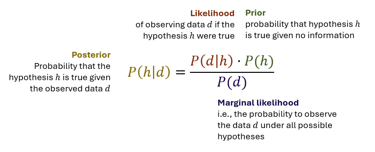
To put this to the test, imagine investigating a static code analysis tool: The tool flags files it considers buggy and should help a company identify actually buggy files. The tool has 90% true positive and 10% false positive rate. Only 5% of files actually have bugs. What’s the probability that a flagged file is buggy?

The quesiton implies two components

• Hypothesis h: a file has a bug
• Data d: a file is flagged as buggy by the static code analysis tool

We are interested in P(h|d), which is exactly the posterior probability. The case description already gives us the likelihood P(d|h) = 0.9 (i.e., the 90% true positive rate) and the prior P(h) = 0.05. We can calculate the marginal likelihood P(d) from the data that we have: P(d) = P(d|h) x P(h) + P(d|-h) x P(-h), which is all available to us, therefore 0.9 x 0.05 + 0.1 x 0.95 = 0.14.

With all components of Bayes’ theorem available, we can calculate P(h|d) = (0.9 x 0.05)/0.14 = 0.321. This means: whenever the tool flags a file as buggy, there is only a 32.1% chance that the file actually contains a bug. This seems counterintuitive at first, but is quite common: If the hypothesis itself has a low probability (prior P(h) = 0.05), then the posterior will also be low despite a high likelihood (i.e., P(d|h) = 0.9) because a majority of the flags that the static code analysis tool produces stem are false positives. The example also illustrates that P(d|h) != P(h|d) and that the difference can actually be very stark.

A Bayesian Workflow

Bayes’ theorem can be used to analyse quantitativ data and answer questions about the probability of hypotheses. In this process, you assign prior probabilities to hypotheses (which represent the existence and strength of the effect of one variable on another) and update these priors with collected data. Richard McElreath has summarized the process in his seminal text book “Statistical Rethinking”¹ covering roughly the following steps:

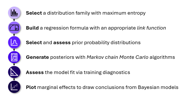
But there is even more to it. Bayesian data analysis lets you adequately model the distribution of a variable (and not just distinguish between normal and non-normal distributions), deal with missing, censored, or truncated data, model hierarchical and interaction relationships, and much more. But most importantly of all: it answers the right question.

Go Bayesian

Learning new methods is tough, and software engineering researchers rarely find the time to improve methodological rigor. But producing results with unreliable conclusion validity is no feasible alternative: If we researchers want to realize our potential and contribute useful and reliable knowledge to software engineering practitioners, we must hone our craft. Bayesian data analysis is one way of improving the conclusion validity of our results, and excellent text books¹ as well as a newly-forming research community around aid the process.

If you are interested in learning more about Bayesian data analysis, do not hesitate to reach out to us. You can find the material from the RE’26 tutorial publicly available on GitHub.²

---