26 Aug 2026
Analysis methods for quantitative data are dominated by frequentist null-hypothesis significance tests (NHSTs) in software engineering research.
Tests like the Student’s t-test, the Kruskal-Wallis-test, or the Mann-Whitney-U-test are convenient tools to tease a conclusion out of a set of data.
Yet, software engineering researchers rarely have the time to question, critique, and improve these methods.
In our tutorial at the 2026 requirements engineering conference, we shed light on these methods and encouraged researchers of all levels of seniority to adopt more valid and sophisticated ones.
P-Values are not the Answer
NHSTs are convenient because they produce a simple p-value which researchers compare with an arbitrarily chosen significance level.
But what exactly is a p-value?
A p-value is the probability of observing data at least as extreme as what you actually got, assuming the null hypothesis is true.
As such, the p-value is a statement about observed data, it is not a statement about the formulated hypothesis.
However, the question of interest is usually: how likely is there an effect of one variable on another?
The p-value does not answer this question.
But there is an answer to this question.
The Bayesian Paradigm
Consider a hypothesis h and observed data d.
The abovementioned definition of a p-value can be translated into the conditional probability P(d|h), i.e., the probability of observing d given h is true.
Yet, what we are after is the conditional probability P(h|d), i.e., the probability that the hypothesis is true given the observed data.
This so-called posterior probability maps much better to the questions researchers are interested in: how likely is an effect between two variables (i.e., hypothesis h) given the data we observed (d) in our study?
We can calculate this posterior probability thanks to Bayes’ theorem and the following components:
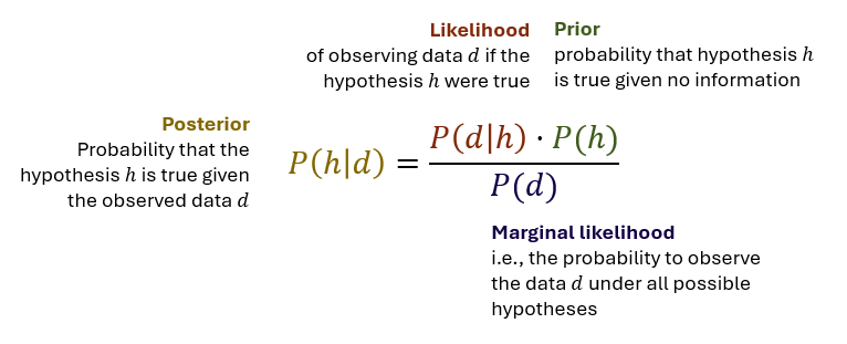
To put this to the test, imagine investigating a static code analysis tool:
The tool flags files it considers buggy and should help a company identify actually buggy files.
The tool has 90% true positive and 10% false positive rate.
Only 5% of files actually have bugs.
What’s the probability that a flagged file is buggy?
The quesiton implies two components
- Hypothesis
h: a file has a bug
- Data
d: a file is flagged as buggy by the static code analysis tool
We are interested in P(h|d), which is exactly the posterior probability.
The case description already gives us the likelihood P(d|h) = 0.9 (i.e., the 90% true positive rate) and the prior P(h) = 0.05.
We can calculate the marginal likelihood P(d) from the data that we have:
P(d) = P(d|h) x P(h) + P(d|-h) x P(-h), which is all available to us, therefore 0.9 x 0.05 + 0.1 x 0.95 = 0.14.
With all components of Bayes’ theorem available, we can calculate P(h|d) = (0.9 x 0.05)/0.14 = 0.321.
This means: whenever the tool flags a file as buggy, there is only a 32.1% chance that the file actually contains a bug.
This seems counterintuitive at first, but is quite common:
If the hypothesis itself has a low probability (prior P(h) = 0.05), then the posterior will also be low despite a high likelihood (i.e., P(d|h) = 0.9) because a majority of the flags that the static code analysis tool produces stem are false positives.
The example also illustrates that P(d|h) != P(h|d) and that the difference can actually be very stark.
A Bayesian Workflow
Bayes’ theorem can be used to analyse quantitativ data and answer questions about the probability of hypotheses.
In this process, you assign prior probabilities to hypotheses (which represent the existence and strength of the effect of one variable on another) and update these priors with collected data.
Richard McElreath has summarized the process in his seminal text book “Statistical Rethinking” covering roughly the following steps:
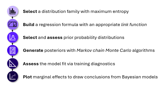
But there is even more to it.
Bayesian data analysis lets you adequately model the distribution of a variable (and not just distinguish between normal and non-normal distributions), deal with missing, censored, or truncated data, model hierarchical and interaction relationships, and much more.
But most importantly of all: it answers the right question.
Go Bayesian
Learning new methods is tough, and software engineering researchers rarely find the time to improve methodological rigor.
But producing results with unreliable conclusion validity is no feasible alternative:
If we researchers want to realize our potential and contribute useful and reliable knowledge to software engineering practitioners, we must hone our craft.
Bayesian data analysis is one way of improving the conclusion validity of our results, and excellent text books as well as a newly-forming research community around aid the process.
If you are interested in learning more about Bayesian data analysis, do not hesitate to reach out to us.
You can find the material from the RE’26 tutorial publicly available on GitHub.
11 Jun 2026
Most scientific manuscripts describing empirical studies in software engineering (SE) - particularly those reporting controlled experiments - almost ritualistically acknowledge threats to external validity in their discussion section.
Like a preemptive defense mechanism against an overly critical reviewer 2, authors backpedal on their claims with excuses like “Because our sample of subjects is limited, we cannot generalize the results.”
Acknowleding this limitation is important, but not even striving for some level of generalizability runs the risk of producing isolated results with negligible usability and relevance to practice.
So when is the external validity of a result actually threatened?
And is acknowledging all that we can do about it?
Understanding Threats to External Validity
Many studies in SE aim to quantify the effect of an independent variable x on a dependent variable y (called the average treatment effect), e.g., the effect of using LLM-support (x) on the productivity of developers (y).
Since it is impossible to involve all software engineers or artifacts in any empirical study, we need to draw a sample to involve in a study.
External validity is the ability to transport the results from this experimental sample to the much larger target population, i.e., the group of people, artifacts, etc. that we want to reason about.
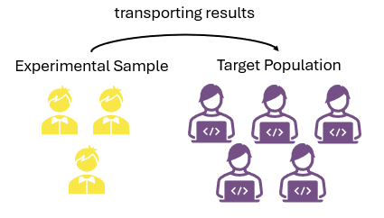
External validity is “our ability to generalize the results of our experiment to industrial practice” (Wohlin, C., Runeson, P., Höst, M., Ohlsson, M. C., Regnell, B., & Wesslén, A. (2012). Experimentation in software engineering (Vol. 236, p. P3). Berlin: Springer.)
So what actually threatens external validity?
There is a surprisingly straight-forward answer to this question.
The external validity of the results from an empirical study are threatened when two conditions hold:
- the average treatment effect of x on y is moderated by a third covariate z, and
- this covariate’s distribution differs in the experimental sample from the target population.
Perfectly clear, right?
Certainly, this may not be straightforward.
So let’s break these conditions down.
Presence of a Moderator
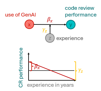
A moderator, or treatment effect modifier, is a third variable z that changes the effect that x has on y.
If no moderator is present, then the effect of x on y is consistent across all levels of z.
But if z acts as a moderator, the effect that x has on y is dependent on the value of z, i.e., it changes over the range of values of z.
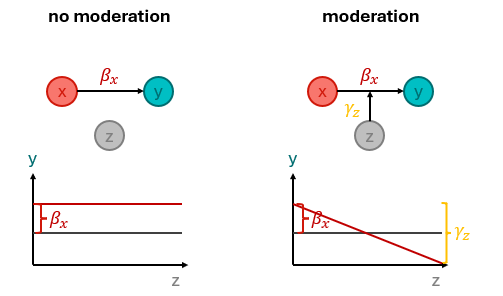
Consider the following example:
When studying the effect that GenAI-usage (x) has on code-review performance (y), the experience of the code reviewer (z) may moderate the effect.
Inexperienced code reviewers (i.e., low values of z) might benefit strongly from the use of GenAI (i.e., experience a positive effect) because GenAI-support is better than nothing.
However, experienced code reviewers (i.e., high values of z) may actually be hindered by GenAI-support (i.e., experience a negative effect) because GenAI-suggestions may be slightly off, confusing, or no match for their domain experience.
In such a case, z moderates the effect of x on y.
Different Distributions
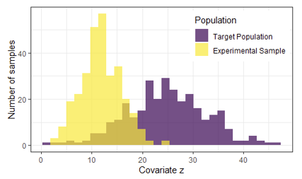
The second condition implies a covariate shift, i.e., that the distribution of a variable is different in a sample from a target population.
This happens very easily in SE studies.
For example, students are easier to recruit than practitioners, but then the covariates experience and skill will differ in the experimental sample from the target population.
Co-Occurrence of both Conditions
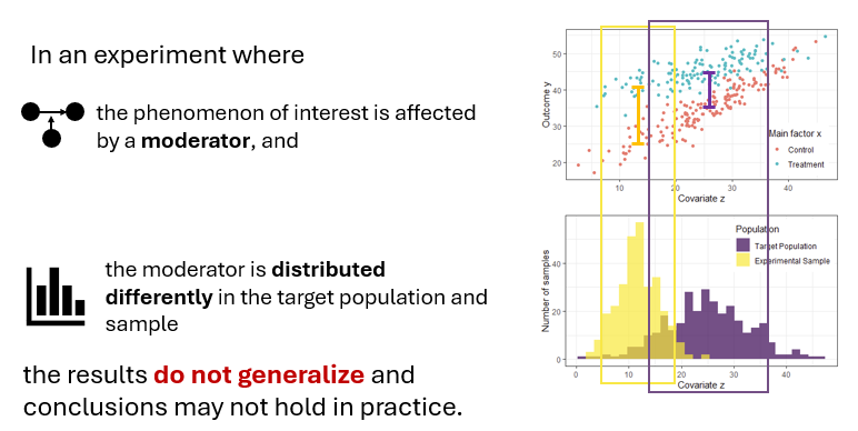
When these two conditions co-occur, i.e., the moderator is also subject to a covariate shift, then we have a threat to external validity.
If our experimental sample focuses only on a particular subset of the target population (e.g., very junior code reviewers) for whom the effect is particularly strong due to the moderator (see the yellow box in the figure below), then the average treatment effect calculated from the experiment will overestimate the effect as it would manifest in the total target population, where the covariate is distributed differently.
Mitigating the Threat to External Validity
But is acknowledging them the only thing we can do?
Turns out, there are statistical techniques to improve the external validity of a controlled experiment as long as
- we collect data about the moderator in question, and
- we have data about the distribution of this moderator from the target population.
The latter could be an observational data set just containing data about z.
Picking up the previous example, it could be a sample study recording the experience in number of years working as a code reviewer of a larger target population (e.g., a company-wide profile).
When this data is available, we can apply transportability methods.
In essence, these work by re-weighting the data points collected in the controlled experiment based on the sampling probability:
when a data point has a covariate value z that is rare in the experimental sample but common in the target population, then it will be weighted much stronger in the estimation of the average treatment effect than a data point where z is common in the experimental sample and rare in the target population.
For example, a few more senior code reviewers in a controlled experiment will influence the results much more than the many students, because these more senior subjects represent the target population much better than the juniors.
Application
How can you use this?
Arguably, the application of these transportability methods is non-trivial, but there are some direct applications available to you today:
- Discussing threats to validity: The presented concepts provide a frame to discuss threats to external validity. Whenever acknowledging threats to external validity in your empirical studies, check: is it plausible to assume that the two conditions (moderator & covariate shift) are present? If not - and if reviewer 2 can also not provide evidence for it - then there might just be no threat to external validity, and critique of your study unjustified.
- Studying threats to validity: If you design an empirical study and have reasons to assume that a (potentially covariate-shifted) moderator is at play, be sure to collect data about it in your study. By visualizing the effects of x on y across z, you can visually confirm this hypothesis and actually bring evidence to the claim.
- Improving validity: Once you have collected your data and you also obtained data about the distribution of the covariate in the target population (e.g., via a survey or MSR-type study), you can apply transportability methods to improve the external validity of your results, effectively producing more relevant conclusions from your research.
A tutorial and library to apply transportability methods is on our agenda and will be published soon.
A note on the final application: we anticipate that collecting (observational) data about the distribution of a moderating covariate will become a very worthwhile research activity given the framework of transportability.
Once we become more aware of what moderators typically affect phenomena in SE research (e.g., developers experience and skill, their AI affinity, etc.), census-style data characterizing our target population could become reusable across several empirical studies for the purpose of transportability.
We envision a productive, collaborative future in empirical SE research when adhering to this frame.
Conclusion
Not every factor threatens external validity, only when it acts as a moderator and is distributed differently than in the intended target population.
If we want to aim for useful and relevant results in SE, we should
- systematically investigate the presence and effect of moderators on SE phenomena, and
- recruit samples accordingly, i.e., try to maximize the coverage of the moderators,
in order to minimize or mitigate threats to external validity.
We hope
We presented this work at the International Conference on Evaluation and Assessment in Software Engineering (EASE) 2026 in beautiful Glasgow, Scotland, where our paper received the “Best Paper Award” on the Short Papers and Emerging Results track.
You can find a publicly accessible pre-print on arxiv at https://doi.org/10.48550/arXiv.2604.08200.
with Transportability Methods. In Proceedings of the 31st International Conference on Evaluation and Assessment in Software Engineering.
https://doi.org/10.48550/arXiv.2604.08200.
27 Oct 2025
At the 2025 International Requirements Engineering Conference, I had the chance to host a tutorial titled Applied Statistical Causal Inference in Requirements Engineering.
The topic of statistical causal inference is very dear to my heart and sharing some fundamental insights with the requirements engineering community, the community closest to my research, was a wonderful opportunity to teach and learn.
In this debriefing, my colleagues and I summarize the main points of the tutorial.
For participants, we hope this helps digesting the material.
For those that missed the tutorial, the following summary may contain some relevant insights and may even get them interestested to join next time around.
Motivation
As any scientific discipline, the software engineering (SE) research community strives to contribute to the betterment of the target population of our research: software producers and consumers.
We will only achieve this betterment if we manage to transfer the knowledge acquired during research into practice.
This transferal of knowledge may come in the form of tools, processes, and guidelines for software developers.
However, the value of these contributions hinges on the assumption that applying them causes an improvement of the development process, user experience, or other performance metrics.
Such a promise requires evidence of causal relationships between an exposure or intervention (i.e., the contributed tool, process or guideline) and an outcome (i.e., performance metrics).
A straight-forward approach to obtaining this evidence is via controlled experiments in which a sample of a population is randomly divided into a group exposed to the new tool, process, or guideline, and a control group.
However, such randomized control trials may not be legally, ethically, or logistically feasible.
In these cases, we need a reliable process for statistical causal inference (SCI) from observational data.
Causal Modelling
Much will be won if researchers in SE adopt one of the simplest techniques in scope of SCI: causal modeling.
We can visualize causal assumptions in the form of directed acyclic graphs (DAGs), where nodes represent variables and directed edges represent assumed causal relationships.
Vice versa, the absence of an edge represents the assumptions that two variables are not directly related.
The figure below shows a simple DAG representing the causal assumption that AI-support affects coding performance.
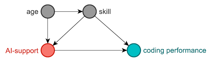
Additionally, the figure encodes the assumption that the skill of a developer both affects their inclination to use AI-support and their overall coding performance.
Similarly, age is assumed to affect skill but also the aforementioned inclination.
Do you agree with this DAG?
You might not.
Based on your assumptions, experience, or prior research, you may find additional variables relevant or you would connect them differently.
A DAG always represents a researcher’s understanding of real-world phenomena.
But a DAG makes this understanding transparent and captures even complex relationships that may not be easily expressed in a null-hypothesis stated in natural language.
Its transparency allows to review, critique, and improve it by proposing the inclusion of new or exclusion of existing variables, and updating the edges between them.
Try to think of other variables that you believe or know would affect the effect of AI-support on coding performance.
In fact, DAGs encourage challenging them:
SCI has methods to determine which one of several potential DAGs reflects the real-world phenomenon better.
This way, we can incrementally improve our understanding of these phenomena.
Three Elemental Sources of Bias
Moreover, DAGs expose potential sources of bias.
In observational studies, the effect of a treatment of interest (here: AI-support) on an outcome of interest (here: coding performance) may be biased by other variables.
This does not happen in true controlled experiments where the treatment is assigned at random.
In a DAG, this would mean that no arrow “enters” (i.e., points towards) the treatment.
But when you understand how other factors bias this effect of interest, you can take counter measures.
There are essentially three different relationships in which a third variable z can interact with an effect of interest of x → y, visualized as the three DAGs below.

These three different types of relationship require different treatment:
- Confounder: If z is a common cause of both x and y (x ← z → y) we must control for it statistically when estimating the effect x → y (where “controlling for” means including the variable in a statistical analysis, for example as a regressor in a linear model). Otherwise, z will bias this effect. This is the classic case of confounding.
- Mediator: If z is located on a pipe (i.e., a causal chain where information flows sequentially from one variable to the next) from x to y (x → z → y) we can control for it. If we do control for z, we distinguish the direct effect (x → y) from the indirect effect through z (x → z → y). If we do not control for z, we obtain the total effect (i.e., combining the direct (x → y) with the indirect (x → z → y) effect). Both are correct, but answer different questions.
- Collider: If z is a common effect of both x and y (x → z ← y) we must not control for it. By default, the effect x → y is unbiased in this case, but controlling for z will introduce a bias. You may know this phenomenon as Berkson’s paradox.
Handling these relationships is a major aspect of research design.
Controlling confounders ensures internal validity, while ignoring colliders makes
sure one does not condition on post-treatment variables.
Controlling mediators allows isolating the direct effect of a treatment.
For example: does a newly proposed testing technique x really improve test coverage y (i.e., the direct effect x → y) or does it rather affect testers’ attention z which in turn produces tests with better coverage (i.e., the indirect effect x → z → y)?
Depending on which effect is stronger, a study may conclude either to employ
the testing technique or heighten the attention of testers.
Overall Framework
Understanding potential sources of bias enables debiasing a causal effect of interest even when dealing with data from an observational study.
The following framework proposed by Julien Siebert (derived from the seminal work of Judea Pearl) includes three steps for SCI:
- Modeling: Formalize your causal assumptions in a DAG.
- Identification: Given the relationships between variables, identify those that you need to statistically control for in order to de-bias the causal effect of interest.
- Estimation: Estimate the causal effect of interest with statistical means (e.g., regression models) while controlling for the previously identified variables.
Adherence to SCI principles will propel our scientific endeavors in SE research beyond limitations of correlational analyses and the constraints of experimentation.
Beyond the ability to de-bias a causal effect of interest, SCI principles contribute further benefits to a scientific discipline:
- The transparency of causal assumptions facilitates iterative improvement of empirical evidence. Reviewing, improving, and comparing causal DAGs maps individual pieces of evidence to the continuous improvement of our understanding of SE phenomena.
- The identification of variables potentially biasing an effect of interest informs data collection, i.e., which factors z to record in addition to x and y such that we can control for them in the analysis.
- Causal DAGs facilitate a clearer and more honest discussion of threats to validity. Instead of relying on common practice, threats to internal validity can be connected to variables that bias the effect of interest but could not be collected.
This is a complex topic one should not expect to master in a day.
Proper SCI is much more powerful but also takes much more effort than just picking an appropriate null-hypothesis significance test.
We hope the tutorial and\or this debriefing inspired you to get into SCI for SE.
In case of questions, we are more than happy to support you in learning more about it.
Resources
Finally, find some useful resources to consult when undertaking the journey of learning SCI.
The publications of many great authors in the recent years have made SCI fairly accessible to the interested researcher:
- “The Book of Why” by Judea Pearl is written for a general audience and masterfully introduces the fundamental ideas, history, and methods of SCI.
- “Statistical Rethinking” by Richard McElreath is the extensive text book teaching the craft of SCI in minute detail. On top of being grounded in causal principles, the author adopts a Bayesian perspective to data analysis.
- “A Crash Course in Good and Bad Controls” by Carlos Cinelli and colleagues elaborates which variables to control for given a causal DAG. Thanks to several illustrative examples, this is a very accessible and rewarding read.
- “Applications of Statistical Causal Inference in Software Engineering” by Julien Siebert summarizes prior work using SCI in SE. This literature study shows that its application is yet limited - meaning that it is the perfect time to get started and join the frontier of SCI in SE.
- “Applying Bayesian Analysis Guidelines to Empirical Software Engineering Data” by Carlo Furia and colleagues applies SCI principles in SE research. This is one of the best practical demonstrations of SCI for our field.
- “Causal Models in Requirement Specifications for Machine Learning: A vision” by Hans-Martin Heyn and colleagues goes even further and applies SCI principles not only to SE research, but to SE practice as well, underlining their overall potential.
Many more great references could be mentioned here, and we hope that many more great references will be added to the list in the future to help our requirements and software engineering community adopt methods of SCI in our portfolio.
For actual application and tooling, we recommend the programming language R and the following packages:
- To draw and evaluate DAGs, we can recommend DAGitty or GGDag.
- To estimate causal effects based on DAGs using a Bayesian perspective, consider following along the above-referenced book “Statistical Rethinking” using the rethinking package. Once having understood the principles, we can recommend switching to brms by Paul Bürkner.
The material from our tutorial remains available under an open source license on GitHub (see: github.com/JulianFrattini/bda4sci).
It includes the presentation slides as well as code examples to recreate figures and analyses.
Finally, you can find an archived version of this blog post on arXiv at arxiv.org/abs/2511.03875.
specifications for machine learning: A vision. In Proceedings of the 33rd ACM In-
ternational Conference on the Foundations of Software Engineering, pages 1402–1405, 2025